A Sample of 12 Babies Was Randomly Selected and the Information Shown Below Was Generated
six.three: The Sample Proportion
- Page ID
- 571
Learning Objectives
- To recognize that the sample proportion \(\hat{p}\) is a random variable.
- To empathize the meaning of the formulas for the mean and standard difference of the sample proportion.
- To learn what the sampling distribution of \(\chapeau{p}\) is when the sample size is big.
Frequently sampling is done in order to estimate the proportion of a population that has a specific characteristic, such as the proportion of all items coming off an assembly line that are defective or the proportion of all people entering a retail store who make a buy before leaving. The population proportion is denoted \(p\) and the sample proportion is denoted \(\hat{p}\). Thus if in reality \(43\%\) of people entering a store make a purchase before leaving,
\[p = 0.43 \nonumber\]
if in a sample of \(200\) people entering the store, \(78\) brand a purchase,
\[\hat{p}=\dfrac{78}{200}=0.39. \nonumber\]
The sample proportion is a random variable: it varies from sample to sample in a way that cannot exist predicted with certainty. Viewed as a random variable information technology will be written \(\hat{P}\). It has a hateful \(μ_{\lid{P}}\) and a standard difference \(σ_{\hat{P}}\). Here are formulas for their values.
mean and standard deviation of the sample proportion
Suppose random samples of size \(due north\) are drawn from a population in which the proportion with a characteristic of involvement is \(p\). The mean \(μ_{\chapeau{P}}\) and standard departure \(σ_{\hat{P}}\) of the sample proportion \(\chapeau{P}\) satisfy
\[μ_{\hat{P}}=p\]
and
\[σ_{\hat{P}}= \sqrt{\dfrac{pq}{n}}\]
where \(q=ane−p\).
The Fundamental Limit Theorem has an analogue for the population proportion \(\hat{p}\). To see how, imagine that every element of the population that has the characteristic of interest is labeled with a \(i\), and that every element that does not is labeled with a \(0\). This gives a numerical population consisting entirely of zeros and ones. Conspicuously the proportion of the population with the special characteristic is the proportion of the numerical population that are ones; in symbols,
\[p=\dfrac{\text{number of 1s}}{N}\]
Just of course the sum of all the zeros and ones is merely the number of ones, so the mean \(μ\) of the numerical population is
\[μ=\dfrac{ \sum 10}{Due north}= \dfrac{\text{number of 1s}}{North}\]
Thus the population proportion \(p\) is the same as the mean \(μ\) of the corresponding population of zeros and ones. In the same way the sample proportion \(\hat{p}\) is the same every bit the sample hateful \(\bar{ten}\). Thus the Central Limit Theorem applies to \(\hat{p}\). Withal, the condition that the sample be big is a little more complicated than just existence of size at to the lowest degree \(30\).
The Sampling Distribution of the Sample Proportion
For big samples, the sample proportion is approximately normally distributed, with hateful \(μ_{\hat{P}}=p\) and standard deviation \(\sigma _{\hat{P}}=\sqrt{\frac{pq}{due north}}\).
A sample is big if the interval \(\left [ p-3\sigma _{\hat{p}},\, p+3\sigma _{\hat{p}} \right ]\) lies wholly within the interval \([0,i]\).
In actual practice \(p\) is not known, hence neither is \(σ_{\hat{P}}\). In that instance in club to check that the sample is sufficiently big we substitute the known quantity \(\lid{p}\) for \(p\). This means checking that the interval
\[\left [ \hat{p}-3\sqrt{\frac{\hat{p}(1-\hat{p})}{n}},\, \hat{p}+3\sqrt{\frac{\hat{p}(one-\chapeau{p})}{n}} \right ]\]
lies wholly within the interval \([0,1]\). This is illustrated in the examples.
Figure \(\PageIndex{ane}\) shows that when \(p = 0.1\), a sample of size \(15\) is as well small just a sample of size \(100\) is acceptable.
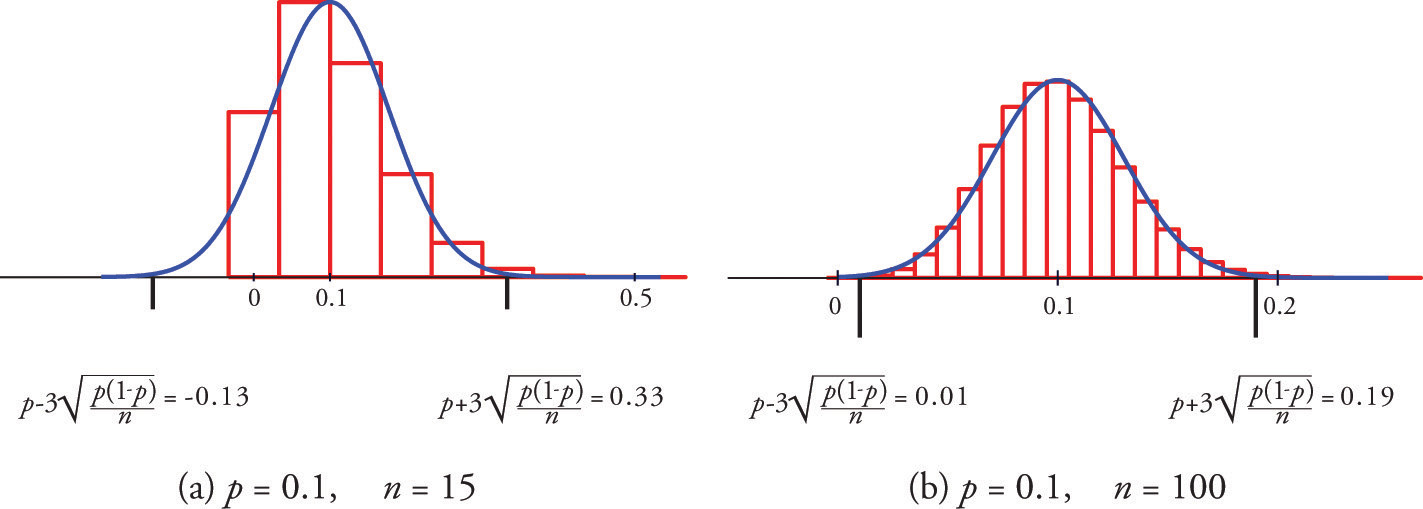
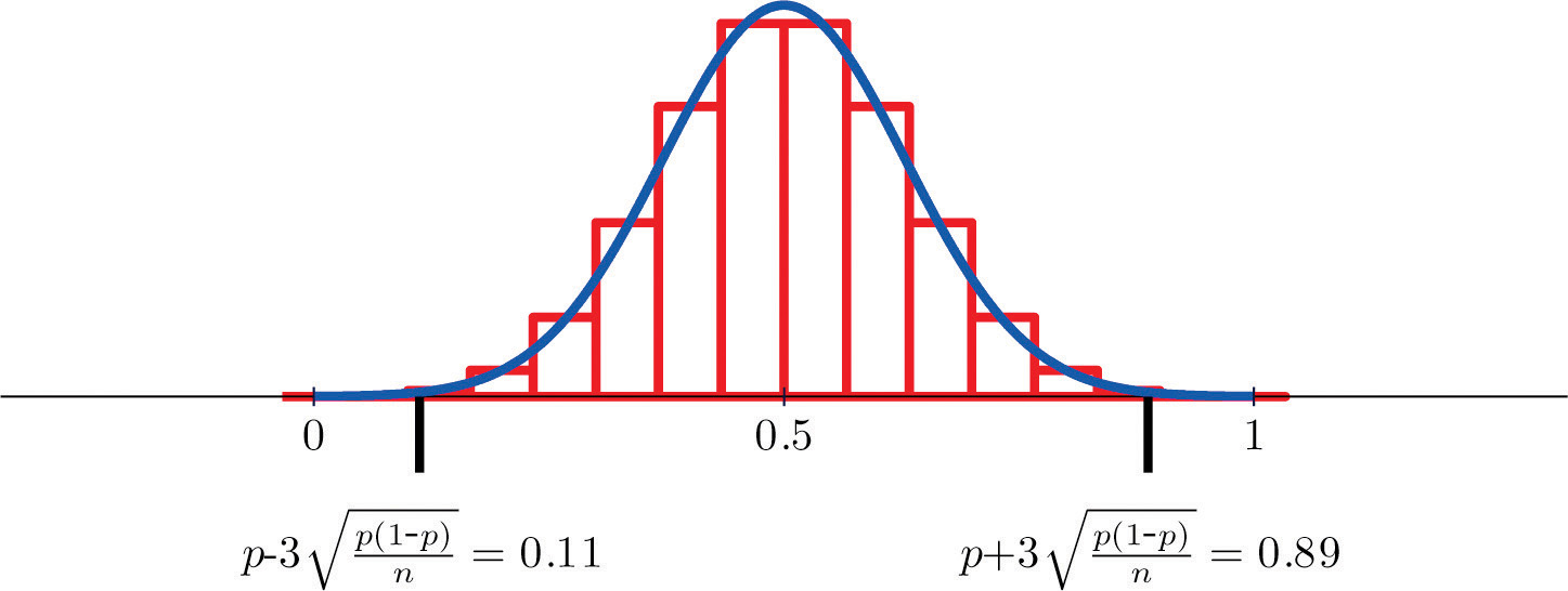
Figure \(\PageIndex{2}\) shows that when \(p=0.5\) a sample of size \(15\) is acceptable.
Example \(\PageIndex{1}\)
Suppose that in a population of voters in a sure region \(38\%\) are in favor of particular bond effect. Nine hundred randomly selected voters are asked if they favor the bond issue.
- Verify that the sample proportion \(\chapeau{p}\) computed from samples of size \(900\) meets the condition that its sampling distribution exist approximately normal.
- Discover the probability that the sample proportion computed from a sample of size \(900\) will be within \(5\) percent points of the true population proportion.
Solution:
- The data given is that \(p=0.38\), hence \(q=1-p=0.62\). Kickoff we use the formulas to compute the hateful and standard deviation of \(\hat{p}\):
\[\mu _{\hat{p}}=p=0.38\; \text{and}\; \sigma _{\lid{P}}=\sqrt{\frac{pq}{northward}}=\sqrt{\frac{(0.38)(0.62)}{900}}=0.01618 \nonumber\]
So \(3\sigma _{\hat{P}}=3(0.01618)=0.04854\approx 0.05\) then
\[\left [ \chapeau{p} - 3\sqrt{\frac{\lid{p}(1-\hat{p})}{northward}},\, \hat{p}+3\sqrt{\frac{\lid{p}(1-\hat{p})}{due north}} \right ]=[0.38-0.05,0.38+0.05]=[0.33,0.43] \nonumber\]
which lies wholly inside the interval \([0,1]\), so it is safe to assume that \(\chapeau{p}\) is approximately normally distributed.
- To be within \(5\) pct points of the true population proportion \(0.38\) ways to exist betwixt \(0.38-0.05=0.33\) and \(0.38+0.05=0.43\). Thus
\[\begin{align*} P(0.33<\lid{P}<0.43) &= P\left ( \frac{0.33-\mu _{\lid{P}}}{\sigma _{\hat{P}}} <Z< \frac{0.43-\mu _{\hat{P}}}{\sigma _{\chapeau{P}}} \right )\\[4pt] &= P\left ( \frac{0.33-0.38}{0.01618} <Z< \frac{0.43-0.38}{0.01618}\right )\\[4pt] &= P(-3.09<Z<three.09)\\[4pt] &= P(3.09)-P(-3.09)\\[4pt] &= 0.9990-0.0010\\[4pt] &= 0.9980 \end{marshal*}\]
Example \(\PageIndex{2}\)
An online retailer claims that \(90\%\) of all orders are shipped within \(12\) hours of being received. A consumer group placed \(121\) orders of different sizes and at unlike times of day; \(102\) orders were shipped within \(12\) hours.
- Compute the sample proportion of items shipped inside \(12\) hours.
- Ostend that the sample is large enough to assume that the sample proportion is normally distributed. Use \(p=0.90\), corresponding to the assumption that the retailer'due south claim is valid.
- Bold the retailer'southward claim is true, find the probability that a sample of size \(121\) would produce a sample proportion so low as was observed in this sample.
- Based on the answer to office (c), describe a conclusion about the retailer's claim.
Solution:
- The sample proportion is the number \(ten\) of orders that are shipped within \(12\) hours divided by the number \(north\) of orders in the sample:
\[\chapeau{p} =\frac{x}{due north}=\frac{102}{121}=0.84\nonumber\]
- Since \(p=0.90\), \(q=1-p=0.x\), and \(n=121\),
\[\sigma _{\lid{P}}=\sqrt{\frac{(0.90)(0.10)}{121}}=0.0\overline{27}\nonumber\]
hence
\[\left [ p-3\sigma _{\hat{P}},\, p+3\sigma _{\hat{P}} \correct ]=[0.90-0.08,0.xc+0.08]=[0.82,0.98]\nonumber\]
Because
\[[0.82,0.98]⊂[0,ane]\nonumber\]
it is advisable to utilize the normal distribution to compute probabilities related to the sample proportion \(\chapeau{P}\).
- Using the value of \(\lid{P}\) from part (a) and the ciphering in part (b),
\[\brainstorm{align*} P(\hat{P}\leq 0.84) &= P\left ( Z\leq \frac{0.84-\mu _{\chapeau{P}}}{\sigma _{\hat{P}}} \right )\\[4pt] &= P\left ( Z\leq \frac{0.84-0.xc}{0.0\overline{27}} \correct )\\[4pt] &= P(Z\leq -2.20)\\[4pt] &= 0.0139 \stop{align*}\]
- The computation shows that a random sample of size \(121\) has only about a \(1.4\%\) chance of producing a sample proportion equally the one that was observed, \(\hat{p} =0.84\), when taken from a population in which the bodily proportion is \(0.90\). This is so unlikely that it is reasonable to conclude that the actual value of \(p\) is less than the \(xc\%\) claimed.
Key Takeaway
- The sample proportion is a random variable \(\chapeau{P}\).
- There are formulas for the mean \(μ_{\hat{P}}\), and standard departure \(σ_{\hat{P}}\) of the sample proportion.
- When the sample size is large the sample proportion is normally distributed.
smithmarjohishe00.blogspot.com
Source: https://stats.libretexts.org/Bookshelves/Introductory_Statistics/Book%3A_Introductory_Statistics_(Shafer_and_Zhang)/06%3A_Sampling_Distributions/6.03%3A_The_Sample_Proportion
0 Response to "A Sample of 12 Babies Was Randomly Selected and the Information Shown Below Was Generated"
Post a Comment